- Published on
🧠 AI Exploration #4: Regression in Supervised Learning
- Authors

- Name
- Van-Loc Nguyen
- @vanloc1808
🧠 AI Exploration #4: Regression in Supervised Learning
In this post, we take a deeper dive into one of the fundamental branches of supervised learning: regression. If you've ever tried to predict house prices, stock values, or the temperature for tomorrow, you're working with regression.
Let’s explore what regression is, how it works, the types of regression algorithms, loss functions, evaluation metrics, and practical use cases.
📐 What is Regression?
Regression is a supervised learning task where the target variable is continuous rather than categorical. The model learns the relationship between input variables (features) and a numerical output.
In contrast to classification, where we predict labels, in regression we predict real-valued numbers.
🏡 Example: Predicting House Prices
Imagine we want to predict the price of a house based on features like:
- Square footage
- Number of bedrooms
- Neighborhood rating
Each training sample contains both the features (input) and the actual sale price (output). The model learns to map feature combinations to a continuous target value.
🧠 Common Regression Algorithms
| Algorithm | Description | Suitable For |
|---|---|---|
| Linear Regression | Models a linear relationship between features and output | Quick baselines, interpretable models |
| Polynomial Regression | Extends linear regression with polynomial terms | Nonlinear trends |
| Ridge / Lasso Regression | Linear regression with regularization to prevent overfitting | High-dimensional data |
| Decision Tree Regressor | Splits input space to minimize variance in each region | Simple nonlinear relationships |
| Random Forest Regressor | Ensemble of trees for robust regression | Tabular data with complex interactions |
| Neural Networks | Multi-layer models with nonlinear activations | Complex, high-dimensional data (e.g., images) |
🧮 Loss Functions
To measure how good our predictions are, we use loss functions.
🔹 Mean Squared Error (MSE)
- Penalizes larger errors more strongly
- Sensitive to outliers
🔹 Mean Absolute Error (MAE)
- Less sensitive to outliers
- More interpretable (same unit as output)
🔹 Huber Loss
- Combines MSE and MAE; quadratic for small errors, linear for large ones
📊 Evaluation Metrics
Once trained, we evaluate regression models using:
| Metric | Description |
|---|---|
| R² Score (Coefficient of Determination) | Measures proportion of variance explained by model |
| RMSE (Root Mean Squared Error) | Square root of MSE; same unit as output |
| MAE | Average absolute error |
| MAPE | Mean Absolute Percentage Error (percentage-based) |
A good regression model should generalize well — low error on both training and validation data.
🧪 Hands-On Project: Predicting Car Prices
A sample dataset might include:
- Input Features: Age, mileage, brand, engine size, fuel type
- Target Output: Sale price in USD
You can use scikit-learn to build:
- A
LinearRegressionmodel - Evaluate using
mean_squared_errorandr2_score - Visualize predictions vs. actuals
Tip: Always check residual plots to ensure your model isn’t systematically wrong.
✅ When to Use Regression
Use regression when:
- Your output is a real number (e.g., price, length, temperature)
- You care about the magnitude of error
- The relationship between input and output might be linear or nonlinear
❗ Common Pitfalls
- Overfitting with complex models (especially on small datasets)
- Ignoring outliers, which can distort the model
- Failing to normalize or preprocess features (especially with gradient-based models)
🧪 Code Example: Simple Linear Regression in Python
We'll create a synthetic dataset with a linear relationship and train a LinearRegression model using scikit-learn.
import numpy as np
import matplotlib.pyplot as plt
from sklearn.linear_model import LinearRegression
from sklearn.metrics import mean_squared_error, r2_score
from sklearn.model_selection import train_test_split
# 🎯 Generate synthetic data
np.random.seed(42)
X = 2 * np.random.rand(100, 1)
y = 4 + 3 * X + np.random.randn(100, 1) # Linear relationship with noise
# 🔀 Split into training and testing sets
X_train, X_test, y_train, y_test = train_test_split(X, y, test_size=0.2, random_state=42)
# 🧠 Train a Linear Regression model
model = LinearRegression()
model.fit(X_train, y_train)
# 📈 Make predictions
y_pred = model.predict(X_test)
# 📊 Evaluate the model
mse = mean_squared_error(y_test, y_pred)
r2 = r2_score(y_test, y_pred)
print(f"Mean Squared Error: {mse:.2f}")
print(f"R² Score: {r2:.2f}")
print(f"Learned parameters: Intercept = {model.intercept_[0]:.2f}, Coefficient = {model.coef_[0][0]:.2f}")
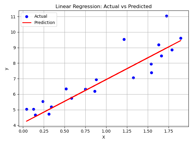
# 📉 Plot the results
plt.scatter(X_test, y_test, color='blue', label='Actual')
plt.plot(X_test, y_pred, color='red', linewidth=2, label='Prediction')
plt.xlabel('X')
plt.ylabel('y')
plt.title('Linear Regression: Actual vs Predicted')
plt.legend()
plt.grid(True)
plt.tight_layout()
plt.show()
🔍 The plot below shows a clear linear trend: the red line (predicted values) closely follows the blue dots (actual values), indicating that the model has successfully captured the underlying relationship despite some noise in the data.
🔚 Recap
Regression is a core tool in the ML toolbox for any problem involving numeric prediction. By understanding the data, selecting the right model, and evaluating it carefully, you can build reliable predictive systems for real-world impact.
🔜 Coming Next
Next in the AI Exploration series: Classification — where we tackle the problem of assigning labels to inputs like spam detection, image recognition, and medical diagnosis.
Stay curious and keep exploring 👇
🙏 Acknowledgments
Special thanks to ChatGPT for enhancing this post with suggestions, formatting, and emojis.