- Published on
Uninformed Searching Strategies
- Authors

- Name
- Van-Loc Nguyen
- @vanloc1808
There are many ways to solve problem with a computer. The primary condition for solving a problem is that we must successfully represent the problem. This post discusses about uninformed searching strategies, which means, we have no other information than the conditions of the problem.
Representation of Search Problems
A problem typically contains requirements and solution. Searching is used to find out the solution in the search space.
A searching problem usually contains five components:
- State space: all possible states of the problem.
- Initial state: the state from which the search starts, for example, the person will start from Ho Chi Minh City.
- Transition model: a function that takes a state and returns a set of states that can be reached from the given state.
- Goal state: the state that we want to reach, for example, the person wants to go to Hanoi.
- Path cost: a function that assigns a numeric cost to each path.
State space
In order to solve a searching problem, we need to define the appropriate state space. Based on the initial state and transition model, we can determine all reachable states, so we can understand that the state space is all reachable states from the initial state.
The state space is usually represented by a graph, so we call state space graph. In this graph:
- Each node represents a state.
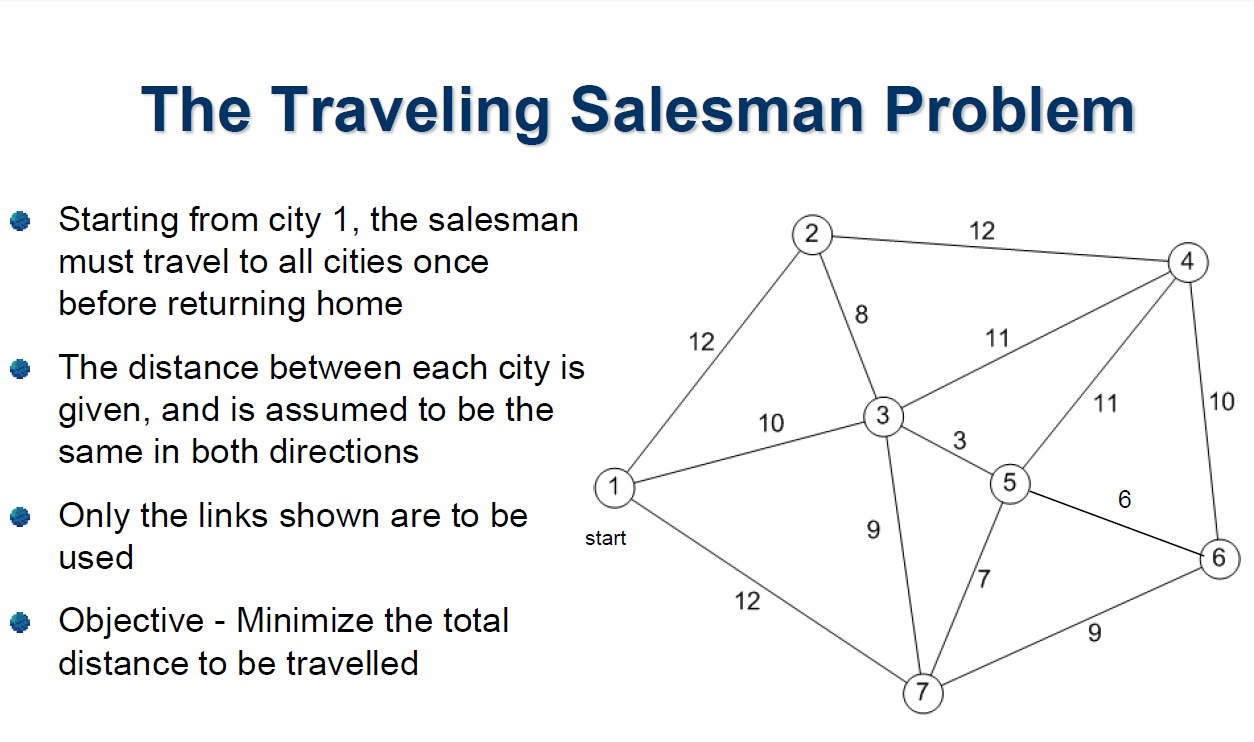
- Each edge represents a transition from one state to another. For example, consider the Traveling Salesman Problem. Its graph representation is as follow.
State
State in the searching problem is the representation of the problem at a particular point in time. The state is represented by a node in the state space graph.
For example, in the Traveling Salesman Problem, a state is a city that the salesman is currently in.
Transition model
The transition model is a function that takes a state and returns a set of states that can be reached from the given state. The transition model is represented by the edges in the state space graph.
Path cost
The path cost is a function that assigns a numeric cost to each path. The path cost is represented by the cost (weight) of the edges in the state space graph.
Searching Problem Examples
The Traveling Salesman Problem (TSP)
The Traveling Salesman Problem is a classic optimization problem. The problem is to find the shortest possible route that visits each city exactly once and returns to the original city.
8-queen Problem
The 8-queen problem is a classic problem in which the goal is to place 8 queens on an 8x8 chessboard so that no two queens threaten each other.
Breadth-First Search (BFS)
Breadth-First Search (BFS) is the expansion of the search tree on breadth. The root node will be initially considered, after that, all the child nodes of the root node will be expanded. Then, all the child nodes of the child nodes of the root node will be expanded, and so on. The Python implementation of the BFS algorithm is as follows:
def bfs(graph, start, goal):
    explored = []
    queue = [[start]]
    if start == goal:
        return "Start is the goal"
    while queue:
        path = queue.pop(0)
        node = path[-1]
        if node not in explored:
            neighbors = graph[node]
            for neighbor in neighbors:
                new_path = list(path)
                new_path.append(neighbor)
                queue.append(new_path)
                if neighbor == goal:
                    return new_path
            explored.append(node)
    return "No path found"
Uniform-Cost Search (UCS)
One of the main disadvantages of BFS is that it does not consider the cost of the path. Uniform-Cost Search (UCS) is an extension of BFS that considers the cost of the path. The Python implementation of the UCS algorithm is as follows:
def ucs(graph, start, goal):
    explored = []
    queue = [[start]]
    if start == goal:
        return "Start is the goal"
    while queue:
        path = queue.pop(0)
        node = path[-1]
        if node not in explored:
            neighbors = graph[node]
            for neighbor in neighbors:
                new_path = list(path)
                new_path.append(neighbor)
                queue.append(new_path)
                if neighbor == goal:
                    return new_path
            explored.append(node)
            queue = sorted(queue, key=lambda x: sum(x))
    return "No path found"
Depth-First Search (DFS)
Unlike BFS, Depth-First Search (DFS) expands the search tree on depth. The Python implementation of the DFS algorithm is as follows:
def dfs(graph, start, goal):
    explored = []
    stack = [[start]]
    if start == goal:
        return "Start is the goal"
    while stack:
        path = stack.pop()
        node = path[-1]
        if node not in explored:
            neighbors = graph[node]
            for neighbor in neighbors:
                new_path = list(path)
                new_path.append(neighbor)
                stack.append(new_path)
                if neighbor == goal:
                    return new_path
            explored.append(node)
    return "No path found"
Iterative Deepening Search (IDS)
Iterative Deepening Search (IDS) is a combination of BFS and DFS. It can optimize the time complexity of BFS and the space complexity of DFS. The Python implementation of the IDS algorithm is as follows:
def ids(graph, start, goal):
    for depth in range(1, len(graph)):
        result = dls(graph, start, goal, depth)
        if result:
            return result
    return "No path found"
References
https://www.geeksforgeeks.org/state-space-search-in-ai/ https://stanford-cs221.github.io/autumn2024/ Artificial Intelligence: A Modern Approach, Stuart Russell and Peter Norvig
Contact
If you have any questions or feedback, feel free to contact me.